Introduction

In the first of this two-part series, we implemented Prometheus client instrumentation within a .Net 6 API application.

In this part, our focus turns to the creation of RED method dashboards. These dashboards will monitor critical metrics such as error rate, request duration, and request rate. To achieve this, we first verify if Prometheus is effectively scrapping data from our API's metrics endpoint. Once confirmed, we'll utilize the power of the Prometheus Query Language (PromQL) to create the dashboards in Grafana.

The RED method serves as a good indicator of user satisfaction. As an example, a high error rate translates directly to user-facing page load errors, impacting user experience. On the other hand, a high request duration rate may signify a slow website, which also affects the user experience.

Audience

To complete this tutorial, you must have a basic understanding of Docker, REST APIs, and System Monitoring.

Prerequisites

To follow along, you will need the following:

.Net6 SDK and runtime installation on your local machine.
Postman or any other REST client installation on your local machine.
Clone the source code and troubleshooting guide here.
Docker installation on your local machine.

Once you have finished the setup, you can continue with this article.

Architecture

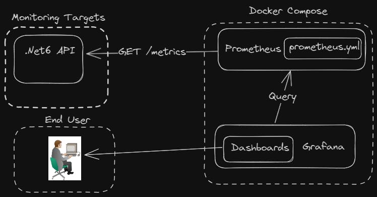
This is what we are going to build:

Prometheus and Grafana

Prometheus is an open-source tool that collects metrics data and provides tools to visualize the collected data. Prometheus operates through the identification of targets, predominantly focusing on HTTP endpoints in the majority of instances. These endpoints can take multiple forms: they might be natively exposed by a component, instrumented within code, or exposed by a Prometheus exporter.

Grafana is an open-source analytics and visualization platform designed to work with various data sources, allowing users to create, explore, and share dashboards. In this tutorial, we will use Prometheus as the primary data source for Grafana. Both tools will be deployed using docker-compose, as outlined below:

version: "3"

services:

  grafana:
    restart: always
    container_name: grafana
    image: grafana/grafana:10.2.0
    ports:
      - 3000:3000
    volumes:
      - grafanadata:/var/lib/grafana

  prometheus:
    restart: always
    container_name: prometheus
    image: prom/prometheus:v2.47.2 
    privileged: true
    volumes:
      - ./docs/config/prometheus.yml:/etc/prometheus/prometheus.yml
      - prometheusdata:/prometheus

    command:
      - '--config.file=/etc/prometheus/prometheus.yml'
      - '--web.enable-admin-api'
      - '--web.enable-lifecycle'
    ports:
      - 9090:9090

volumes:
  grafanadata:
  prometheusdata:

Let's go through the docker-compose file:

services: This file defines two services, named grafana and prometheus.
restart: always: Both services are configured to automatically restart in case of any container stoppage.
volumes: Containers for both services should attach volumes for data persistence. For example, the service prometheus attaches the volume prometheusdata to the container path prometheusdata. Volume attachment, in this case, ensures that scraped data remains available even after a container restart.
.docs/config/prometheus.yml:/etc/prometheus/prometheus.yml: This line mounts the local prometheus.yml configuration file to the container on the path /etc/prometheus/prometheus.yml. This mapping is essential due to the read-only nature of the default configuration file, located at /etc/prometheus/prometheus.yml. Therefore, changes must be propagated through a local configuration file. If you have cloned the source code, you will recognize this path from your sources.
ports: Containers for both services should map a local port to a port in the container. For example, the service grafana maps port 3000 of the host machine to port 3000 in the Grafana container. Port mapping, in this case, enables localhost access to Grafana's web interface.
command: [...]: This specifies the command arguments that will be passed when initiating the Prometheus container.
--web.enable-lifecycle: This command enables a reload of the configuration file without restarting Prometheus.

Let's spin up the containers and ensure everything is working:

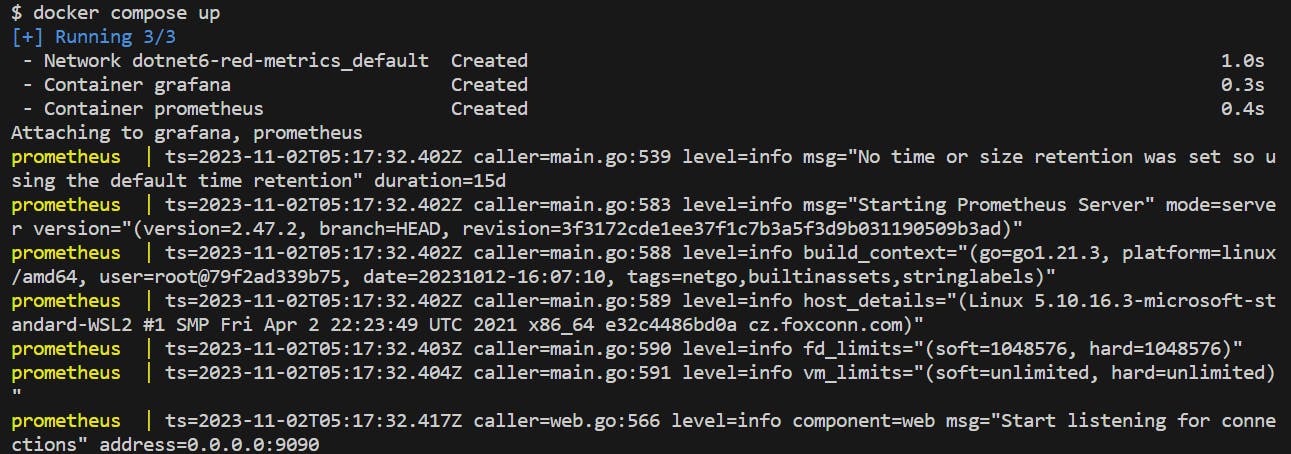
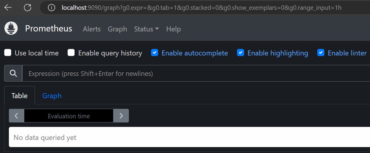
If Prometheus is up it should be accessible on http://localhost:9090/ :

If Grafana is up it should be accessible on localhost:3000. Unlike the Prometheus UI, which by default operates without authentication, Grafana UI requires that you provide a valid username and password for access. The default login credentials for Grafana are provided below:

Username –> admin
Password –> admin

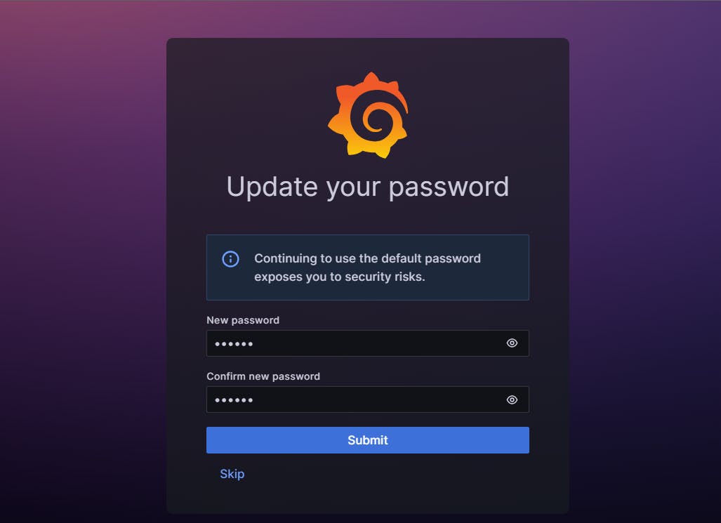
If you have not modified the Grafana version in the docker-compose, you will be prompted to enter a new password as illustrated below:

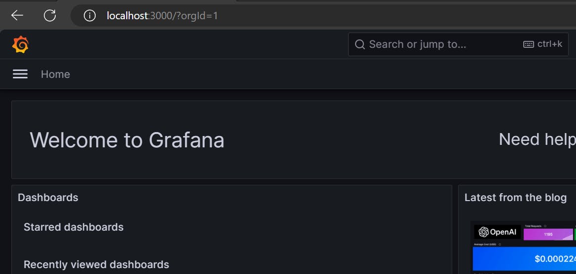
After a successful login, you will be presented with a screen like below:

NOTE: Use docker compose up to start the services defined in the docker-compose.yml file and docker-compose down to stop the services.

Step 1 - Register Metrics endpoint with Prometheus

When registering targets in Prometheus, the approach you select depends on your server and client architecture.

There are several methods to consider:

Static Configuration via prometheus.yml.
Service Monitors and Kubernetes Label Filters.
Dynamic Service Discovery.
Target-Pushed Metrics for Prometheus.

Given that we have a Docker compose installation, we will opt for the static configuration method. This method involves updating the configuration file prometheus.yml. If you have cloned the source code, you will recognize this file at the path blogs\dotnet6-red-metrics\docs\config.

Now, let's add our metrics endpoint as a target:

global:
  scrape_interval: 15s # Set the scrape interval to every 15 seconds. Default is every 1 minute.
  evaluation_interval: 15s # Evaluate rules every 15 seconds. The default is every 1 minute.
  # scrape_timeout is set to the global default (10s).
# Alertmanager configuration
alerting:
  alertmanagers:
    - static_configs:
        - targets:
          # - alertmanager:9093
rule_files:
  # - "first_rules.yml"
scrape_configs:
  # The job name is added as a label `job=<job_name>` to any timeseries scraped from this config.
  - job_name: "prometheus"
    static_configs:
      - targets: ["localhost:9090"]
  - job_name: "net6-red-api"
    static_configs:
      - targets: ["localhost:5283"]
  - job_name: "node-api"
    static_configs:
      - targets: ["localhost:3000"]

What we are doing:

scrape_interval: Prometheus scrapes metrics from monitored targets at regular intervals, defined by the scrape_interval. We opt for 15 seconds.
evaluation_interval: This value tells Prometheus how often it should evaluate alerting rules. We are not implementing any alerts, so this parameter is irrelevant for now.
scrape_timeout: The timeout of a scrape is 10 seconds. If a scrape takes longer than the set scrape_timeout, Prometheus will cancel it.
scrape_configs: Scrape configs tell Prometheus where to find targets. We add them by providing a static list of <host>:<port> targets.
job_name: We define a job with the name net6-red-api. This effectively registers our metrics endpoint as a Prometheus target.

Let's verify the changes:

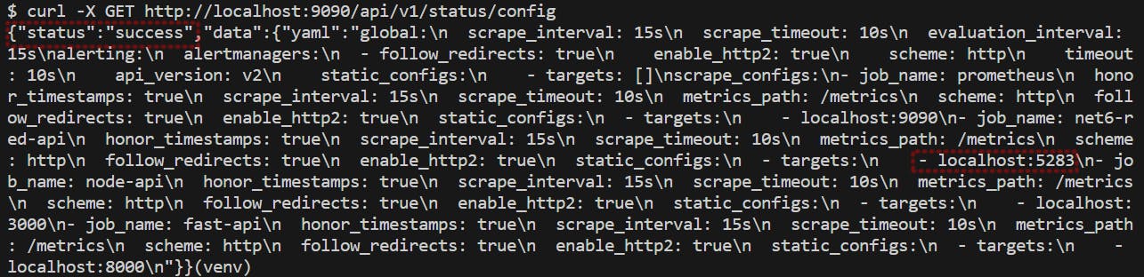
The reload was successful and we can also confirm the addition of our metrics endpoint as a target.

Step 2- Verify API metrics in Prometheus

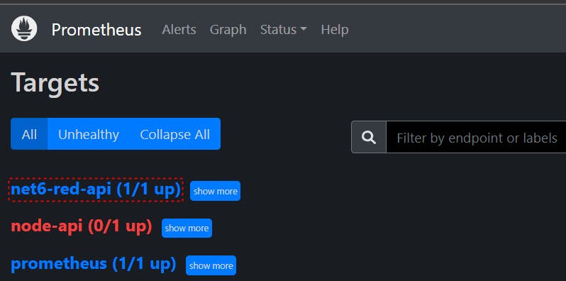
Using the Prometheus UI, we can check if we registered the metrics endpoint. To verify this, go to http://localhost:9090/targets and check if the endpoint is listed under scrape targets:

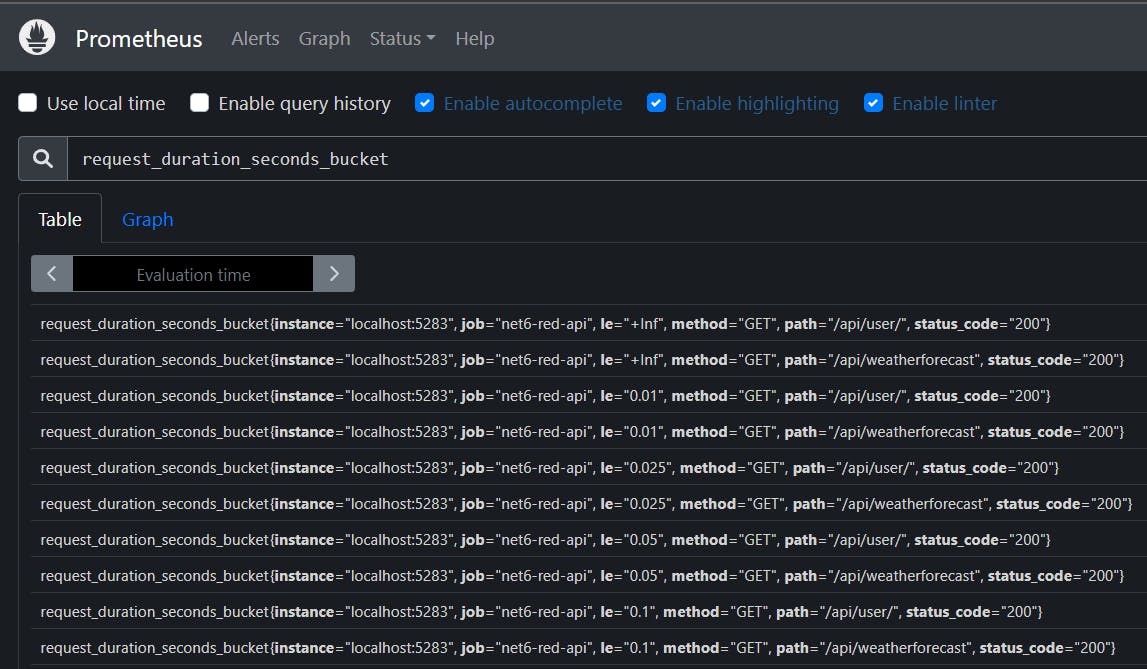
To view the metrics exposed by the API, we use Prometheus's built-in Expression Browser. To do so, navigate to http://localhost:9090/graph and select the "Table" view tab. Enter the metric name and click "Execute":

Step 3 - Configure Prometheus to Grafana Integration

Before we can design dashboards, we must add Prometheus as a data source in Grafana. To set this up, navigate to the Connections icon in the left menu and select Data sources. This action will open a new page, where you can add a new data source. Fill in the fields as illustrated below:

To access the Prometheus server, use the URL "http://prometheus:9090" instead of "localhost:9090". The name "prometheus" in the URL refers to the name of the Prometheus container. Also, make sure both containers are on the same docker network. We are doing so because "localhost", in the context of a container, refers to only what's inside that container (only Grafana is running in the grafana container).

Docker-compose will do three things in this respect:

It automatically creates a docker network on which it attaches the grafana and prometheus containers.
It creates a docker network that is named after the directory of the docker-compose file. The name of the network also has a "default" suffix i.e dotnet6-red-metrics_default. If you have cloned the source code you will recognize this network when you run docker compose up.
It automatically handles DNS resolution between the two containers.

Let's verify this network configuration:

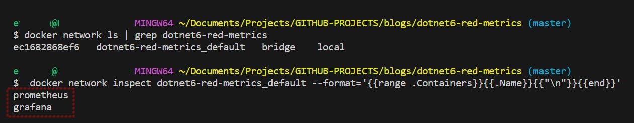
The network ls command lists the available docker networks. Since we already know the pattern of the network name, we add a filter to return just that network. The network inspect command goes through the containers on the network and prints their names.

Step 4 - Configure RED Method Dashboards

With the new data source in place, let’s add the RED dashboard and its corresponding panels. To recap, we are creating a dashboard to track errors, duration, and rate - three key metrics embodying the RED method of observability.

Errors

The Error component of the RED method serves as an accurate indicator of Availability. Availability is the proportion of requests that resulted in a successful response.

To spin up the RED method dashboard we start by adding a panel for the Error metric. We use the request_duration_seconds_metric metric from our API to calculate the Error component. To do so, we make use of the following PromQL query :

sum(increase(request_duration_seconds_count{status_code!="200"}[1m]))/sum(increase(request_duration_seconds_count[1m])) *100

This query calculates the percentage of requests with a non-"200" status code compared to all requests over the past 1 minute, grouped by path.

Let's deconstruct the query :

sum: Add up all the values of the metric selected in the previous 1 minute.
increase: Calculate how much request_duration_seconds_count Counter increased in the specified interval (1 minute here). The Counter's value changes based on the initial (re)start time of the process that tracks and exposes it, so its absolute value is usually not useful. Therefore, before performing any operations on a Counter, we must encapsulate it within a function such as rate(), irate() or increase(). This will enable us to assess the Counter's actual rate of change.
by path: Calculate the sum separately for each unique value of the path label.
status_code: Only consider samples where the HTTP response code is not equal to 200.

We add a special panel for Error Percentage to the dashboard, as demonstrated below:

Let's break down the panel into its key elements:

Gauge: Any time you want to measure a value that fluctuates, opt for a Gauge. For example, the error percentage is a dynamic value that can go up or down over a given time interval.
Unit: Use percentage as the unit of measurement.

To validate the Errors metric, we execute 10 requests within a 1-minute timeframe. It is also important to ensure that the requests are executed within the scrape_interval periods. For example, you can execute 2 requests in every 15 seconds of the 1-minute window. To do this, open Postman and execute the following requests:

localhost:5283/api/weatherforecast (5 requests)
localhost:5283/forecast/problem (5 requests)

The resulting Error rate should be 50%. If you get a different value, be sure to double-check your dashboard configuration and query for any potential inconsistencies.

Rate

The Rate component of the RED method serves as an accurate indicator of Throughput. Throughput refers to the rate at which a system or service can process and handle a certain volume of requests or transactions within a given period.

We use the request_duration_seconds_bucket metric from our API to calculate the Rate component. To do so, we make use of the following PromQL query :

round(sum(rate(request_duration_seconds_bucket[1m0s])), 0.001)

The query calculates the average rate at which requests are being processed per second based on the request duration metric, over a 1-minute interval.

Let's deconstruct the query :

rate(request_duration_seconds_bucket[1m0s]): This computes the per-second rate of change of the request_duration_seconds_bucket within a 1-minute timeframe.
sum(...): We apply the sum function to the result of the rate calculation, which effectively aggregates the rate values over the specified time window.
round(...,0.001): The final step rounds the sum calculation to three decimal places, ensuring a precision of 0.001. This simplifies the data output by removing any unnecessary decimal places.

Duration

The Duration component of the RED method serves as an accurate indicator of Latency. Latency is the proportion of requests that were faster than some threshold. We usually describe latency with its 99th percentile or P99. For example, if we say an API has a P99 latency of 2 milliseconds, then it means that 99% of the requests coming to the API receive a response within 2 milliseconds. Conversely, only 1% of requests experience a delay exceeding 2 milliseconds.

We use the request_duration_seconds_bucket metric from our API to calculate the Duration component. To do so, we make use of the following PromQL query :

query#1
histogram_quantile(0.99, sum(rate(request_duration_seconds_bucket[1m])) by (le, path))

query#2
histogram_quantile(0.9, sum(rate(request_duration_seconds_bucket[1m])) by (le, path))

query#1

Calculates the response times experienced by 99% of all client HTTP requests, over a 1-minute interval.

query#2

Calculates the response times experienced by 90% of all client requests within a given 1-minute interval.

Let's break down the query:

histogram_quantile: Each time Prometheus-net measures the time elapsed between a request and its corresponding response, that’s an observation. The Prometheus server will group these observations into quantiles (or buckets) for us to provide valuable insights.
0.9- This corresponds to the "rank" or "percentile" value, typically within a range of 0 to 1.
rate: Calculate the average per-second increase for each bucket over the past minute, individually.
sum: Combine the increase rates of all buckets over the last minute to obtain an aggregate result.
by (le, path): Count the number of requests based on their duration, and segment them by a specific path. The le denotes less than or equal to.

We add another panel for Request Duration to the dashboard, as demonstrated below:

Let's break down the panel into its key elements:

Time Series: Add a panel of type 'time series'.
Metrics Browser: Include two PromQL queries within the panel: one for the 99th percentile and another for the 90th percentile.
Legend: The legend provides more insight. It ensures that the panel displays the maximum, minimum, and mean duration times.
Unit: Use 'milliseconds (ms)' as the unit of measurement. This choice aligns with our API, which defines a Histogram of ten buckets, ranging from 10 milliseconds through to 10000 milliseconds:

//MetricsReporter.cs
_responseTimeHistogram = Metrics.CreateHistogram("request_duration_seconds",
 "The duration in seconds between the response to a request.", new HistogramConfiguration
  {
     Buckets = new[] { 0.01, 0.025, 0.05, 0.1, 0.25, 0.5, 1, 2.5, 5, 10  },
  });

Summary

That's a wrap 🎉. We have successfully implemented a reference architecture for the RED method. We have only scratched the surface of the RED method here and there is certainly more you can add to make your applications more "observable".

What are some of the lessons you have discovered whilst implementing observability in your applications?

If you liked this article follow me on Twitter for more DevOps, Cloud & SRE.

Ed Tshuma's Blog